hifast.sep processes raw data from a single beam, differentiating raw spectral data when the noise diode is on (Cal on) and off (Cal off). It computes the antenna temperature using noise diode data.
In FAST’s data, each beam’s data is stored in multiple file blocks, named 0001.fits—9999.fits. Input the path of the first file block (e.g., /proj/20211205/XXX_arcdrift-M02_F_0001.fits) to sequentially process these files.
Determine the noise diode switching cycle using three parameters -d,-m,-n, representing delay time, Cal on time, and Cal off time, each divided by the spectral line sampling time. (Example)
These formulas yield the antenna temperature excluding noise diode contributions, requiring noise diode temperature \(T_{\mathrm{cal}}\) and response \(P_{\mathrm{cal}}\).
\(T_{\mathrm{cal}}\): Uses FAST’s official noise diode temperature file.
- --noise_mode: Noise diode strength during observation. Options: high or low; default: high.
- --noise_date: Which day’s noise temperature file to use (e.g., 20190115), see Tcal Data Configuration. If set to auto, selects the nearest file to the observation date.
\(P_{\mathrm{cal}}\): Derived from the noise diode’s Cal_on spectral line power minus the adjacent Cal_off spectral line power. Regular noise diode activations provide a \(P_{\mathrm{cal}}\) each cycle.
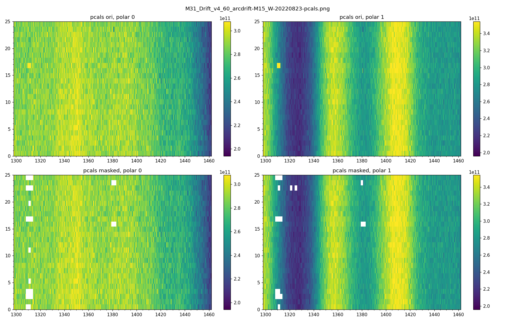
Checking \(P_{\mathrm{cal}}\): (--check_calA, supports if Cal_off sampling number -n is greater than 6).
If a noise diode activates on a continuous spectral source or experiences Radio Frequency Interference (RFI), it can’t be used. The program compares the variation in several Cal_off near Cal_on, with a specific variation threshold. Spectral lines are binned by frequency (--freq_step_c), and bins with Cal_off variation exceeding --pcal_vary_lim_bin are marked damaged. A Cal_on with many damaged bins (--pcal_bad_lim_freq) is discarded. Output includes waterfall charts for verification.
Calibrating each spectral line with \(P_{\mathrm{cal}}\):
Method one: Individual processing (--merge_pcalsFalse).
Each spectral line is calibrated using the nearest \(P_{\mathrm{cal}}\) (smoothed to reduce noise). If the nearest is damaged, it searches for the next undamaged one. If the distance to the nearest Cal_on exceeds --cal_dis_lim, the line’s temperature is marked as nan.
Method two: Merge for frequency dependence (--merge_pcalsTrue).
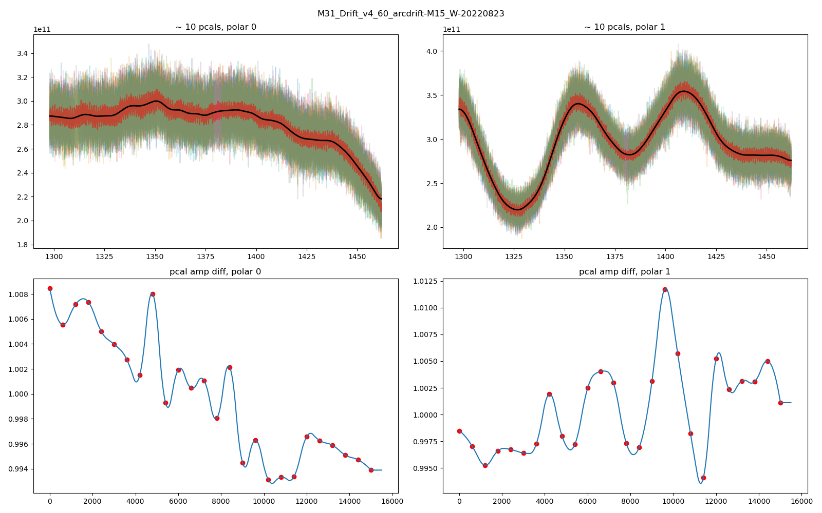
\(P_{\mathrm{cal}}\)’s frequency dependence over time is relatively stable, only varying in amplitude:
\[P_{\mathrm{cal}}(t,\nu) = Amp(t)*F(\nu)\]
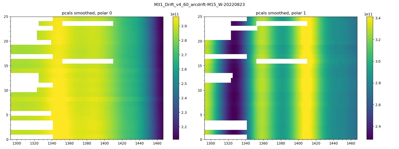
All \(P_{\mathrm{cal}}\) are merged (--method_mergeMergeFun) and smoothed to obtain frequency dependence:
Output images showcase \(P_{\mathrm{cal}}\) variations and interpolation results.
Smoothing parameters (SmooothFun):
- --smooth: Smoothing method options: gaussian, poly, or mean.
- --s_sigma: Required for gaussian smoothing, unit MHz.
- Gaussian smoothing is ideal for large frequency intervals; mean is for smaller intervals; poly fits polynomially with --s_deg.